Neural Graphics Primitives - 1

Introduction

Graphical primitives form the foundation of how we represent complex shapes on a computer —by breaking them down into simpler ones. Take my personal favorite, the movie TRON (1982). Every object in the digital world of TRON—from the light cycles to the voxelized version of Jeff Bridges—was built using basic 3D shapes like cubes, tetrahedrons, cones, and spheres (and their boolean combinations).

Since then, computer graphics has evolved dramatically, but the idea of using primitives still lies at the core of rendering any 3D object onto a 2D screen. You’ve probably seen triangles used to approximate 3D surfaces—they’re the simplest closed shapes with positive area (simplicial complex) and perfectly suited for GPUs to transform from the 3D world to our screens.

Recently, a lot has been happening. Unless you’ve been living under a rock, you’ve probably heard about deep learning and machine learning—and how they’re slowly taking over the world. But not every AI is HAL 9000. Thanks to the rise of neural networks, gradient descent, and all that good stuff, computer graphics has gifted itself two beautiful innovations: NeRFs and Gaussian Splatting. In this blog, I’ll dive into how these modern “primitives” provide powerful new ways to represent models—and the elegant math that makes them work. But before we jump in, let’s take a moment to talk about how graphics used to be done (and is still done).

Rendering

Rendering in computer graphics is the process of transforming a 3D world—much like the one we live in—into a 2D image that appears on a screen from a particular viewpoint. It involves an enormous number of mathematical operations running in parallel to determine how every surface interacts with light and perspective. This is where GPUs shine: they are built to handle thousands of these computations simultaneously. Their ability to perform these calculations at incredible speed is what makes real-time rendering possible in modern video games and simulations.

Broadly speaking, there are two main classes of rendering algorithms: Rasterization and Ray Tracing. Since this blog focuses on understanding how NeRFs work, we’ll primarily explore Ray Tracing. It’s a technique that feels intuitive—rooted in our geometric understanding of how light travels and interacts with objects, without diving into the particle-versus-wave shenanigans.

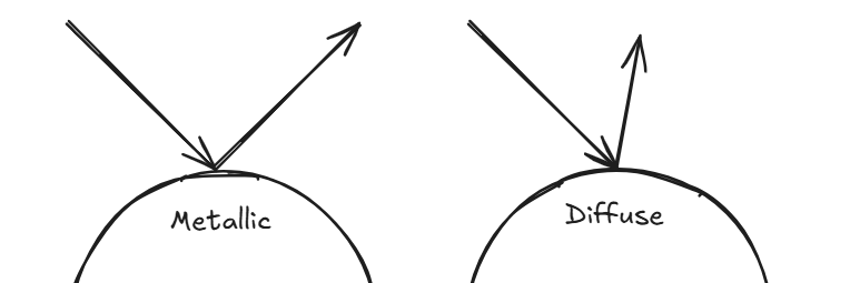
In the physical world, we perceive objects through the light rays that bounce off their surfaces and enter our eyes. These rays originate from sources like the Sun or a light bulb, and the way an object reflects them determines how we see it. For instance, a metallic surface reflects light perfectly—its angle of reflection mirrors the angle of incidence—creating a sharp, mirror-like appearance. In contrast, a rough or diffuse surface scatters light in many directions, giving it a soft, matte look. The proportion of light that’s reflected versus transmitted also shapes how an object appears: if most light is reflected, the object looks opaque; if it’s partly reflected and partly refracted, it appears translucent; and if most light passes through, it becomes transparent.

With this understanding, we can now engineer a method to render an image. Given a light source, an object, and a camera placed at a specific position, the most straightforward idea is to shoot rays from the light source, observe how they interact with the object’s surface based on its material properties—how they reflect, refract, or scatter—and finally collect the rays that end up reaching the camera. In theory, this approach works beautifully and produces highly realistic renderings. But in practice, it’s computationally expensive. Tracing every possible ray from the light source—and accounting for all their reflections and refractions—is simply too heavy to compute, and we have no easy way of knowing how many rays to sample in the first place.

Here’s where a clever trick comes in: since we only care about the rays that actually reach the camera, we can reverse the process. Instead of shooting rays from the light source, we cast them from the camera into the scene and track how they interact with objects. This inversion drastically reduces the number of computations while achieving the same visual effect.

When we want to render something we are just coloring a bunch of pixels on the screen at the end of the day. That is what pixels are for. Each pixel is a unit that shows the color visible to the human eye. The color is represented by the RGB value of a pixel. Every unique proportion of RGB gives a unique color with each channel's value being an integer from 0 to 255 (8bit).

When we set out to render an image of a 3D model, we build upon this understanding of light and pixels. Instead of firing countless rays from the light source, we start right where it matters — the camera. From the camera’s origin, we cast rays that travel through the center of each pixel on the image plane (one such ray is shown below). Each ray is extended into the scene until it intersects an object. Once that happens, the color of the object at the intersection point determines the color of that pixel.

To make the rendering more realistic, we apply basic physics based on the material properties of the surface it hits. If the object is metallic, we reflect the ray and use the color from wherever it bounces next. If it’s transparent, we refract the ray and use the color of what lies beyond. And so on — the principle remains the same. Each ray tells a tiny story of light’s journey through the scene, and together, they paint the final image we see (Sorry to cringe you out!).

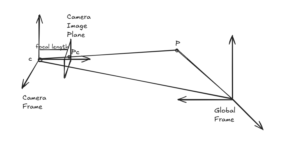
If we view an environment in the global frame, the camera position can be represented as a vector \( \vec{o} \) and vector \( \vec{d} \) pointing from the camera origin to a given pixel representing the direction of the ray. So we can mathematically represent a ray as the vector sum of origin position and the direction vector scaled up to any value (\(t \in \mathbb{R}\)) If you want gain deeper knowledge on ray tracing and would enjoy building your own ray tracer I would suggest checking out Ray Tracing in One weekend



Any rendering algorithm that relies on shooting rays from pixels and coloring them based on their interactions with the scene falls under the broad class of ray tracing methods. Among these, one particularly interesting variant is volume ray casting. This technique becomes extremely useful when the environment we wish to render isn’t made up of solid surfaces, but rather a volumetric field — think of fog, smoke, clouds, or translucent materials — where particles (or the medium) continuously interact with light. 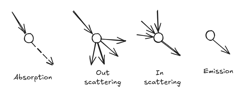A light ray traveling through such a medium can interact with it in four fundamental ways:

• Absorption: The ray loses intensity as light energy is absorbed by the medium.
• Out-scattering: Light is deflected away from the original path.
• In-scattering: Multiple rays are redirected into the ray’s direction, adding brightness.
• Emission: The medium itself emits light from certain regions.

All these interactions collectively influence the intensity of the light as it travels, and this behavior is beautifully captured by a simple but powerful relation known as the Beer–Lambert Law: This equation describes how the intensity \( I(s) \) of a light ray changes as it moves along a path \( s \) through a medium. The parameter \(\sigma\) — often called the optical density — encapsulates the properties of the medium: how much light is absorbed, scattered, or emitted at a given location. Assuming \(\sigma \) is constant, the equation can be solved to give: The ratio above is called transmittance — it represents the fraction of light that successfully passes through the medium without being absorbed or scattered. The above equation is fine as long as the medium is homogeneous i.e. the \(\sigma\) value stays constant. But if we were to deal with hetergenous media (which would be the most common scenario), we have to consider the change in the optical density. So the equation becomes In essence, the farther a light ray travels through a dense medium, the dimmer it becomes, following an exponential decay. Now, when rendering a volumetric medium, we follow the same ray-shooting idea, but instead of finding a single intersection point, we accumulate the light contributions from all points the ray encounters along its path. This becomes an integration of all the transmittance at every given point in space I have written the rendering equation in a very simplified manner. 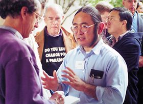To read more on the topic of volume rendering check out this blog. Below I give the equation in its real form and the image of the man - James Kajiya who came up with it

Neural Radiance Fields

Let’s get into the meat and potatoes. Neural Radiance Fields (NeRFs) use neural networks to learn the 3D structure of a scene or object by observing multiple 2D images captured from different viewpoints. This tackles one of the fundamental challenges in photogrammetry — reconstructing accurate 3D geometry from 2D observations. The difficulty arises because, when a 3D scene is projected onto a 2D image, we inherently lose depth information. In simple terms, while an image tells us where things appear, it doesn’t directly tell us how far they are. This relationship is captured by the following formulation: This equation describes how a point in the 3D world \((x,y,z)\) is projected onto a 2D image plane \((u,v)\). The transformation first moves the point into the camera’s coordinate frame through the extrinsic matrix \(R_{4\times4}\) , and then applies the camera intrinsics \(K_{3\times4}\) to project it onto the image plane. As we can see in the transformation, we lose one of the coordinates and there is no direct way we can inverse this process.

where

• \(f_x, f_y\) = Focal lengths
• \(c_x, c_y\) = Camera plane center coordinates

If we could somehow recover this lost depth information, we would gain a complete 3D understanding of the captured scene — enabling us to even recreate images from entirely new viewpoints. A NeRF model achieves this by using multiple images of the same scene taken from different angles. It then trains a neural network to represent the 3D structure and appearance of that scene in a continuous way. In essence, the network learns a function that maps any 3D point and viewing direction to the color and density of light at that location. But how exactly does this network do that? What kind of architecture allows it to learn such complex geometric and visual relationships? Here’s where all the puzzle pieces start to fit together. The rendering equation we discussed earlier will come in handy once again — let’s rewrite it using the notation from the original NeRF paper: where

• \(C\) = net radiance or color value of the pixel
• \(\vec{r}(t)\) = ray passing through a particular pixel center
• \(t_f\) & \(t_n\) = far and near bounds of the scene respectively
• \(\vec{d}\) = viewing direction of the camera (represented in the polar coordinates)

Cool — now that we have this equation, we can approximate \(\sigma\) and \(\mathbf{c}\) using neural networks. According to the paper, NeRF achieves impressive results even with a relatively simple network architecture. They implemented a small MLP with just eight hidden layers — quite minimal compared to many of today’s large-scale models.

Images are sampled from multiple camera viewpoints, allowing rays to intersect the same 3D location from different perspectives. This enables the network to learn both the volume density and the view-dependent color of the scene. The loss function used is a straightforward pixel-wise mean squared error (MSE) loss.

Implementation

I implemented the classical NeRF with positional encoding on a synthetic dataset of the NeRF data - a model of a chair. I trained for 100 epochs on a RTX 4060 with 2048 rays every batch which took around 21 mins with an exponential scheduling on the learning rate and downsampled the image 4 times the actual resolution for faster training while compromising a little on the quality. I have added the training montage below hopefully you find it as mesmerizing as I did.

Below is an inference of novel views of a camera rotating along the x - axis.

The trained sigma model of NeRF acts a indication function of the volume occupied in a given scene that can be used to extract the geometry of the object by using some mesh building algorithm like the marching cubes

Conclusion

Neural Radiance Fields represent a beautiful convergence of geometry, physics, and deep learning — blending classical rendering equations with the representational power of neural networks. What started as a clever mathematical reformulation of volume rendering has now evolved into one of the most elegant ways to reconstruct and render 3D scenes with photorealistic detail.

Unlike traditional graphics pipelines that rely on fixed primitives like triangles or voxels, NeRF learns to represent the scene continuously — as a smooth, differentiable function of space and viewing direction. This not only allows it to capture intricate lighting effects and fine geometry, but also to generalize to new viewpoints with stunning accuracy.

Of course, the classical NeRF is just the beginning. Its successors — Instant NGPs, Mip-NeRF, and Gaussian Splatting — have pushed the limits of speed, quality, and scalability. Yet, the core idea remains the same: using the mathematics of light and density as the foundation, and neural networks as the expressive medium.

The future of computer graphics might not just be about rendering faster or prettier images — but about learning to understand and synthesize reality itself.